Prelims

Magnetic Saturation

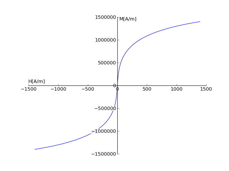
The book Computer-aided Analysis of Electric Machines by Vlado Ostovic uses the Langevin’s function to depict magnetic saturation. Here is a translation of the Mathematica code given in the book to python.


                    from __future__ import division 

                    from functools import partial 

                    from scipy.optimize import fsolve 

                    import numpy as np 

                    import matplotlib.pyplot as plt 

                    import matplotlib as mpl 


                    def coth(x): 

                        return 1/np.tanh(x) 

    
                    def Langevin(M, H): 

                        Ms,a,alpha = 2*10**6,1100,1.6*10**(-3) 

                        return (M/Ms)-(coth((H+alpha*M)/a)-a/(H+alpha*M)) 


                    ms=[] 

                    hs=[] 

                    for m in np.linspace(-14*10**5,14*10**5,5*10**4): 

                        h = fsolve(partial(Langevin,m),-1390) 

                        ms.append(m) 

                        hs.append(h) 


                    ticklabelpad = mpl.rcParams['ytick.major.pad'] 


                    fig = plt.figure(1) 

                    ax = plt.subplot(111) 

                    fig.add_subplot(ax) 

                    ax.spines['right'].set_color('none') 

                    ax.spines['top'].set_color('none') 

                    ax.xaxis.set_ticks_position('bottom') 

                    ax.spines['bottom'].set_position(('data',0)) 

                    ax.yaxis.set_ticks_position('left') 

                    ax.spines['left'].set_position(('data',0)) 

                    ax.annotate('M[A/m]', xy=(.56,1), xycoords='axes fraction', 

                                horizontalalignment='center', verticalalignment='top') 

                    ax.annotate('H[A/m]', xy=(0,.53), xycoords='axes fraction',  

                                horizontalalignment='left', verticalalignment='center') 

                    plt.plot(hs,ms) 

                    for label in ax.get_xticklabels() + ax.get_yticklabels(): 

                        label.set_fontsize(12) 

                        label.set_bbox(dict(facecolor='white', edgecolor='None', alpha=0.65 )) 

                    plt.savefig("sat.png") 

                    plt.show()

The generated plot looks something like this:

I have yet to figure out how to take care of the following warning and the time taken to generate the plot seems too long. Any ideas?


                    In [3]: %run saturation_curve_plot.py 

                            /Users/amaity/.virtualenvs/env1/src/scipy/scipy/optimize/minpack.py:221: 

                            RuntimeWarning: The iteration is not making good progress, as measured by the 
 
                            improvement from the last ten iterations. 

                            warnings.warn(msg, RuntimeWarning)

avamaity

Magnetic Saturation